Every detector on one graph¶

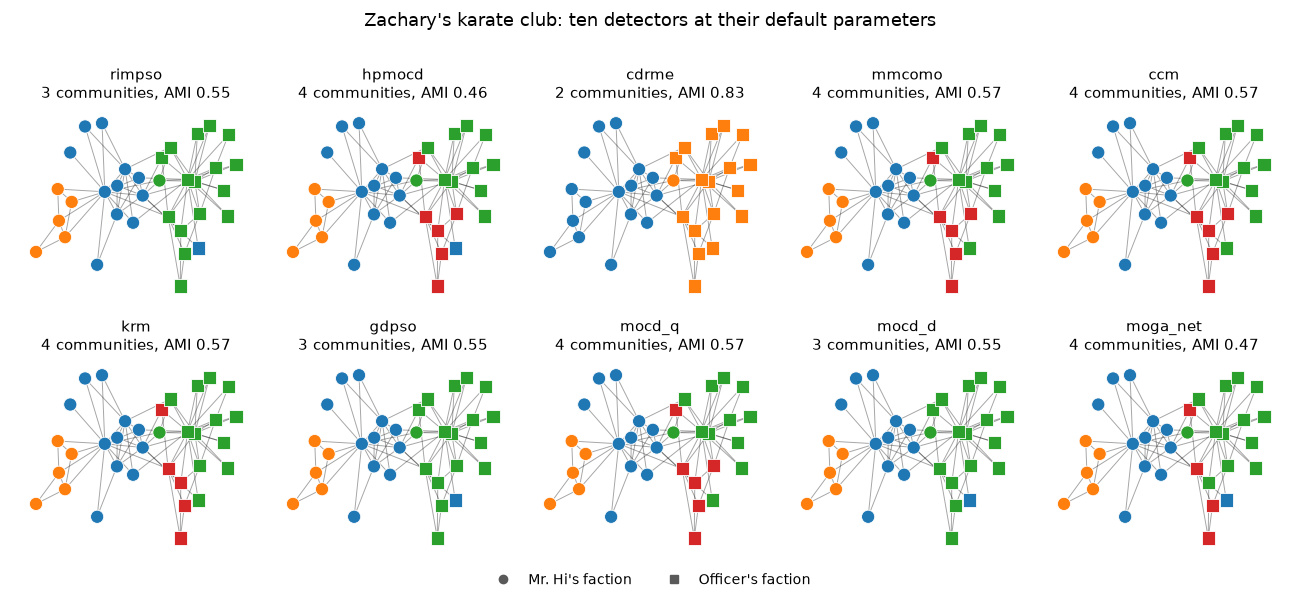
Run all ten detector entry points at their default parameters on Zachary's karate club, draw the ten partitions on one shared layout, and score each against the club's recorded split.

Run the ten detectors¶

Every detector takes the graph as its only required argument and returns a dict mapping each node to a community id. Two are the library's own methods, pymocd.rimpso and pymocd.hpmocd; the other eight entry points implement the seven re-implemented baselines (Shi-MOCD has two, mocd_q and mocd_d): pymocd.cdrme, pymocd.mmcomo, pymocd.ccm, pymocd.krm, pymocd.gdpso, pymocd.mocd_q, pymocd.mocd_d and pymocd.moga_net. The algorithms overview describes each one.

Each detector runs with its own defaults (population size, number of generations and so on differ between them), so this page is a tour of the API, not a benchmark.

import matplotlib.pyplot as plt
import networkx as nx

import pymocd

G = nx.karate_club_graph()
truth = {v: int(G.nodes[v]["club"] != "Mr. Hi") for v in G}

detectors = {
    "rimpso": pymocd.rimpso,
    "hpmocd": pymocd.hpmocd,
    "cdrme": pymocd.cdrme,
    "mmcomo": pymocd.mmcomo,
    "ccm": pymocd.ccm,
    "krm": pymocd.krm,
    "gdpso": pymocd.gdpso,
    "mocd_q": pymocd.mocd_q,
    "mocd_d": pymocd.mocd_d,
    "moga_net": pymocd.moga_net,
}
partitions = {name: detect(G) for name, detect in detectors.items()}

Draw the partitions¶

All panels share one layout. Community ids are arbitrary, so each partition is renumbered in order of its lowest node id before coloring: the community that holds node 0 is always blue, the next one found is orange, and so on. Marker shape shows the recorded split (the club node attribute).

def by_lowest_node(partition):
    """Renumber communities in the order their lowest node id appears."""
    order = {}
    for v in sorted(partition):
        order.setdefault(partition[v], len(order))
    return {v: order[c] for v, c in partition.items()}


pos = nx.spring_layout(G, seed=7)
cmap = plt.colormaps["tab10"]
shapes = {0: "o", 1: "s"}

fig, axes = plt.subplots(2, 5, figsize=(13, 6))
for ax, (name, partition) in zip(axes.flat, partitions.items()):
    colors = by_lowest_node(partition)
    k = len(set(partition.values()))
    ami = pymocd.ami(partition, truth)
    nx.draw_networkx_edges(G, pos, ax=ax, width=0.7, alpha=0.35)
    for side, marker in shapes.items():
        nodes = [v for v in G if truth[v] == side]
        nx.draw_networkx_nodes(
            G,
            pos,
            nodelist=nodes,
            node_color=[cmap(colors[v]) for v in nodes],
            node_shape=marker,
            node_size=90,
            edgecolors="white",
            linewidths=0.6,
            ax=ax,
        )
    ax.set_title(f"{name}\n{k} communities, AMI {ami:.2f}", fontsize=11)
    ax.set_axis_off()

handles = [
    plt.Line2D([], [], marker="o", linestyle="", color="0.35", label="Mr. Hi's faction"),
    plt.Line2D([], [], marker="s", linestyle="", color="0.35", label="Officer's faction"),
]
fig.legend(handles=handles, loc="lower center", ncol=2, frameon=False, fontsize=10)
fig.suptitle("Zachary's karate club: ten detectors at their default parameters", fontsize=13)
fig.tight_layout(rect=(0, 0.05, 1, 0.97))
plt.show()

Zachary's karate club: ten detectors at their default parameters, rimpso 3 communities, AMI 0.55, hpmocd 4 communities, AMI 0.46, cdrme 2 communities, AMI 0.83, mmcomo 4 communities, AMI 0.57, ccm 4 communities, AMI 0.57, krm 4 communities, AMI 0.57, gdpso 3 communities, AMI 0.55, mocd_q 4 communities, AMI 0.57, mocd_d 3 communities, AMI 0.55, moga_net 4 communities, AMI 0.47

Compare against the club split¶

pymocd.gt_metrics returns NMI, AMI, ARI and pairwise F1 against the recorded split in one call.

print(f"{'detector':<10} {'k':>3} {'NMI':>6} {'AMI':>6} {'ARI':>6} {'F1':>6}")
for name, partition in partitions.items():
    k = len(set(partition.values()))
    nmi, ami, ari, f1 = pymocd.gt_metrics(partition, truth)
    print(f"{name:<10} {k:>3} {nmi:>6.3f} {ami:>6.3f} {ari:>6.3f} {f1:>6.3f}")

Out:

detector     k    NMI    AMI    ARI     F1
rimpso       3  0.568  0.551  0.591  0.764
hpmocd       4  0.490  0.464  0.392  0.598
cdrme        2  0.837  0.833  0.882  0.939
mmcomo       4  0.588  0.567  0.465  0.646
ccm          4  0.588  0.567  0.465  0.646
krm          4  0.593  0.571  0.483  0.664
gdpso        3  0.568  0.551  0.591  0.764
mocd_q       4  0.588  0.567  0.465  0.646
mocd_d       3  0.568  0.551  0.591  0.764
moga_net     4  0.498  0.470  0.429  0.634

Reproducibility¶

rimpso (its docstring), cdrme and gdpso (their module READMEs) are deterministic: the same graph, with its nodes and edges listed in the same order, and the same parameters give the same partition (see Input order). The module READMEs of the other seven describe them as nondeterministic, so their panels and rows can change from one build of this page to the next. A single run on a 34-node graph says little about how detectors compare; see Choosing a detector and the benchmark examples for that.

Total running time of the script: ( 0 minutes 1.444 seconds)

Download Python source code: plot_detector_tour.py

Download Jupyter notebook: plot_detector_tour.ipynb

Gallery generated by mkdocs-gallery