Note
Click here to download the full example code
LFR fidelity
Ask pymocd.lfr_graph and NetworkX's
LFR_benchmark_graph for the same LFR graphs, from well-separated to fully
mixed communities, and plot the mixing and the mean degree each generator
actually delivers against the values requested.
The request
Both generators take the same parameters: n = 1000 nodes, degrees from a
power law with exponent tau1 = 3 and requested mean average_degree = 20,
capped at max_degree = 50, and community sizes from a power law with
exponent tau2 = 1.5 between 20 and 100 nodes. Only the mixing mu varies.
NetworkX generates every cell of this sweep. Each target is drawn with three
seeds.
The mixing is measured the way LFR defines it, node by node: the fraction of a node's edges that leave its community, averaged over the nodes. A self-loop, which NetworkX can produce, counts twice toward its node's degree and as an edge inside the community, as NetworkX counts it.
import matplotlib.pyplot as plt
import networkx as nx
import numpy as np

import pymocd

N = 1000
PARAMS = dict(n=N, tau1=3.0, tau2=1.5, average_degree=20, max_degree=50, min_community=20, max_community=100)
TARGETS = [0.0, 0.1, 0.2, 0.3, 0.4, 0.5, 0.6, 0.7, 0.8, 0.9, 1.0]
SEEDS = [1, 2, 3]


def networkx_lfr(mu, seed):
    """networkx.LFR_benchmark_graph as an edge list and a {node: community} dict."""
    G = nx.LFR_benchmark_graph(mu=mu, seed=seed, **PARAMS)
    community = {v: min(G.nodes[v]["community"]) for v in G}
    return list(G.edges()), community


def pymocd_lfr(mu, seed):
    return pymocd.lfr_graph(mu=mu, seed=seed, **PARAMS)


def realized(edges, community):
    """Mean degree, mean node mixing and self-loop count of one graph."""
    degree = np.zeros(N)
    outside = np.zeros(N)
    loops = 0
    for u, v in edges:
        if u == v:
            loops += 1
            degree[u] += 2
            continue
        degree[u] += 1
        degree[v] += 1
        if community[u] != community[v]:
            outside[u] += 1
            outside[v] += 1
    return degree.mean(), (outside / degree).mean(), loops
Generate both sweeps
generators = {"pymocd.lfr_graph": pymocd_lfr, f"networkx {nx.__version__}": networkx_lfr}
shape = (len(TARGETS), len(SEEDS))
mixing = {name: np.full(shape, np.nan) for name in generators}
mean_degree = {name: np.full(shape, np.nan) for name in generators}
loops = {name: np.zeros(shape, dtype=int) for name in generators}
for name, generate in generators.items():
    for i, mu in enumerate(TARGETS):
        for j, seed in enumerate(SEEDS):
            mean_degree[name][i, j], mixing[name][i, j], loops[name][i, j] = realized(*generate(mu, seed))
Plot realized against requested
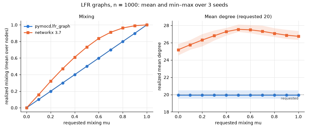
Each line joins the means over the three seeds; the shaded band spans the lowest and highest of them. On the left, the dotted diagonal is where the realized mixing equals the requested one. On the right, the dotted line is the requested mean degree.
style = {
    "pymocd.lfr_graph": {"color": "#2a78d6", "marker": "o"},
    f"networkx {nx.__version__}": {"color": "#eb6834", "marker": "s"},
}
fig, (left, right) = plt.subplots(1, 2, figsize=(10, 4.2))
for name in generators:
    s = style[name]
    for ax, values in ((left, mixing[name]), (right, mean_degree[name])):
        ax.fill_between(TARGETS, values.min(axis=1), values.max(axis=1), color=s["color"], alpha=0.15, linewidth=0)
        ax.plot(TARGETS, values.mean(axis=1), label=name, linewidth=2, markersize=6, **s)
left.plot([0, 1], [0, 1], color="0.4", linestyle=":", linewidth=1.2)
left.set_xlabel("requested mixing mu")
left.set_ylabel("realized mixing (mean over nodes)")
left.set_title("Mixing", fontsize=11)
right.axhline(PARAMS["average_degree"], color="0.4", linestyle=":", linewidth=1.2)
right.text(1.0, PARAMS["average_degree"] - 0.25, "requested", color="0.3", fontsize=8, ha="right", va="top")
right.set_ylim(bottom=PARAMS["average_degree"] - 2)
right.set_xlabel("requested mixing mu")
right.set_ylabel("realized mean degree")
right.set_title(f"Mean degree (requested {PARAMS['average_degree']})", fontsize=11)
for ax in (left, right):
    ax.grid(color="0.9")
    ax.set_axisbelow(True)
    ax.spines[["top", "right"]].set_visible(False)
left.legend(frameon=False, fontsize=9, loc="upper left")
fig.suptitle(f"LFR graphs, n = {N}: mean and min–max over {len(SEEDS)} seeds", fontsize=12)
fig.tight_layout()
plt.show()
The numbers behind the plot
Means over the three seeds; loops is the mean number of self-loops per
graph.
print(f"{'mu':>4}" + "".join(f"  {name:>26}" for name in generators))
print(f"{'':>4}" + "".join(f"  {'mixing  degree  loops':>26}" for _ in generators))
for i, mu in enumerate(TARGETS):
    cells = "".join(
        f"  {mixing[name][i].mean():>12.4f} {mean_degree[name][i].mean():>7.2f} {loops[name][i].mean():>5.0f}"
        for name in generators
    )
    print(f"{mu:>4.1f}{cells}")
Out:
  mu            pymocd.lfr_graph                networkx 3.7
           mixing  degree  loops       mixing  degree  loops
 0.0        0.0000   19.96     0        0.0000   25.18   372
 0.1        0.0999   19.96     0        0.1574   25.76   324
 0.2        0.1992   19.96     0        0.3198   26.31   269
 0.3        0.2997   19.96     0        0.4717   26.80   203
 0.4        0.3992   19.96     0        0.6094   27.28   160
 0.5        0.4995   19.96     0        0.7313   27.55   100
 0.6        0.5992   19.96     0        0.8365   27.49    59
 0.7        0.6998   19.96     0        0.9113   27.32    32
 0.8        0.7991   19.96     0        0.9624   27.08    16
 0.9        0.8984   19.96     0        0.9895   26.87     5
 1.0        1.0000   19.96     0        1.0000   26.74     0
Reading the comparison
pymocd.lfr_graph gives every node exactly the degree it drew, and rounds
each node's internal degree (1 - mu) k up or down at random, so its curve
follows the diagonal up to rounding noise. Its degree law has the requested
mean exactly, so its mean degree scatters around the request by sampling
noise alone. Here it does not change with mu either: a seed's draw of
degrees comes before anything that depends on mu, and every call in this
sweep is wired from its first draw (see
Benchmark graphs).
NetworkX wires one node at a time and compares a node's whole degree, edges
attached by other nodes included, with its internal target, so a node wired
late can meet that target with external edges. It also draws each new
neighbour without checking whether that neighbour already has its full degree
(networkx#6809). Degrees
therefore end above the drawn ones, and for every mu strictly between 0 and 1
the mixing ends above the request; at 0 and 1 no edge can go the wrong way.
The minimum degree NetworkX derives from average_degree is a separate source
of error in its mean degree. The guide page explains both, and
Recovery as mixing increases shows how a detector's
score depends on the mixing.
Total running time of the script: ( 0 minutes 3.070 seconds)
Download Python source code: plot_lfr_fidelity.py