RIMPSO's resolution profile¶

Build a graph with communities at two scales, compute RIMPSO's Pareto front with pymocd.rimpso_fronts, read the front as the graph's resolution profile, and see which member the label-free selector returns.

A graph with structure at two scales¶

A stochastic block model with nine blocks of 15 nodes. The blocks come in three groups of three, called super-blocks here. Two nodes in the same block are joined with probability 0.6, two nodes in different blocks of the same super-block with probability 0.1, and any other pair with probability 0.005. The graph therefore has two planted partitions: nine blocks (fine) and three super-blocks (coarse). NetworkX records each node's block in the block node attribute.

import matplotlib.pyplot as plt
import networkx as nx
import numpy as np
from matplotlib.colors import LinearSegmentedColormap, LogNorm
from matplotlib.ticker import NullLocator

import pymocd

n_super, blocks_per_super, block_size = 3, 3, 15
p_block, p_super, p_out = 0.6, 0.1, 0.005

n_blocks = n_super * blocks_per_super
probs = [
    [
        p_block if a == b else p_super if a // blocks_per_super == b // blocks_per_super else p_out
        for b in range(n_blocks)
    ]
    for a in range(n_blocks)
]
G = nx.stochastic_block_model([block_size] * n_blocks, probs, seed=1)

blocks = {v: G.nodes[v]["block"] for v in G}
super_blocks = {v: blocks[v] // blocks_per_super for v in G}
n, m = G.number_of_nodes(), G.number_of_edges()
print(f"{n} nodes, {m} edges, {n_blocks} blocks in {n_super} super-blocks")

Out:

135 nodes, 795 edges, 9 blocks in 3 super-blocks

Compute the front¶

pymocd.rimpso_fronts runs the same search as pymocd.rimpso and returns the whole archive: a list of partitions, the (cut, pair) point of each, and the index of the member that rimpso returns. cut is the fraction of edges that leave their community and pair the fraction of node pairs that share one; both are minimized. The graph is sampled with a fixed seed and RIMPSO is deterministic (the same graph and parameters give the same result), so the front and the numbers below are the same on every run with the same versions of pymocd and NetworkX.

partitions, points, selected = pymocd.rimpso_fronts(G)
cut = np.array([c for c, _ in points])
pair = np.array([p for _, p in points])
k = np.array([len({c for c in p.values() if c != -1}) for p in partitions])

print(f"front members: {len(partitions)}, from {k.min()} to {k.max()} communities")
print(f"selected member: {selected}, {k[selected]} communities")

Out:

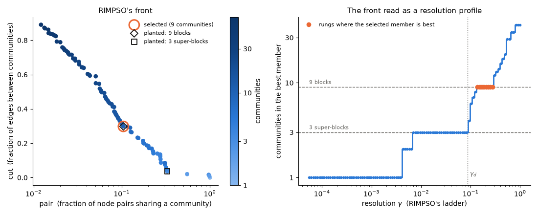
front members: 98, from 1 to 66 communities
selected member: 3, 9 communities

The front is the resolution profile¶

The Constant Potts Model (CPM) at resolution \(\gamma\) scores a partition by \(H_\gamma = \sum_c [e_c - \gamma \binom{n_c}{2}]\), where \(e_c\) is the number of edges inside community \(c\) and \(n_c\) its number of nodes. With the edge density \(\gamma_d = m / \binom{n}{2}\),

\[ H_\gamma = m \left[ 1 - \mathrm{cut} - \frac{\gamma}{\gamma_d}\, \mathrm{pair} \right], \]

so maximizing CPM at any \(\gamma\) is minimizing \(\mathrm{cut} + (\gamma / \gamma_d)\, \mathrm{pair}\). Every resolution is one weighting of the same two objectives, which is why the RIMPSO docstring and module README call the \((\mathrm{cut}, \mathrm{pair})\) front the graph's resolution profile; Core concepts gives the derivation.

RIMPSO's swarm places one particle on each rung of a ladder of pop_size resolutions spaced geometrically over \([1/n^2, 1]\) (the RIMPSO module README calls it the resolution ladder). The code below rebuilds that ladder and, at every rung, finds the front member that minimizes the weighted sum: the best partition the front holds for CPM at that \(\gamma\). A member that is best at no rung does not appear on the right-hand curve; the code prints how many members are best at some rung.

pop_size = 100  # rimpso's default
gamma_d = m / (n * (n - 1) / 2)
gammas = float(n) ** (2 * np.linspace(0, 1, pop_size) - 2)  # n^(2t - 2), t in [0, 1]
best = np.argmin(cut[None, :] + (gammas[:, None] / gamma_d) * pair[None, :], axis=1)
print(f"{len(set(best.tolist()))} of {len(partitions)} front members are the best member at some rung")

# (cut, pair) of the two planted partitions, as rimpso_select reports them.
_, planted_points = pymocd.rimpso_select(G, [blocks, super_blocks])

BLUE, ORANGE, AQUA, INK, MUTED = "#2a78d6", "#eb6834", "#1baf7a", "#1a1a19", "#6b6a66"
ramp = LinearSegmentedColormap.from_list(
    "blues", ["#86b6ef", "#5598e7", "#2a78d6", "#1c5cab", "#104281", "#0d366b"]
)

fig, (ax_front, ax_profile) = plt.subplots(1, 2, figsize=(11, 4.4))

sc = ax_front.scatter(pair, cut, c=k, cmap=ramp, norm=LogNorm(vmin=1, vmax=k.max()), s=28, zorder=2)
ax_front.scatter(
    pair[selected], cut[selected], s=220, facecolors="none", edgecolors=ORANGE,
    linewidths=2.2, zorder=3, label=f"selected ({k[selected]} communities)",
)
for (pc, pp), marker, label in zip(
    planted_points, ["D", "s"], [f"planted: {n_blocks} blocks", f"planted: {n_super} super-blocks"]
):
    ax_front.scatter(pp, pc, marker=marker, s=60, facecolors="none", edgecolors=INK,
                     linewidths=1.4, zorder=4, label=label)
ax_front.set_xscale("log")
ax_front.set_xlabel("pair  (fraction of node pairs sharing a community)")
ax_front.set_ylabel("cut  (fraction of edges between communities)")
ax_front.set_title("RIMPSO's front", fontsize=11)
ax_front.legend(loc="upper right", fontsize=8, frameon=False)
k_ticks = [t for t in (1, 3, 10, 30, 100) if t <= k.max()]
cbar = fig.colorbar(sc, ax=ax_front, label="communities")
cbar.set_ticks(k_ticks, labels=[str(t) for t in k_ticks])
cbar.ax.minorticks_off()

ax_profile.plot(gammas, k[best], color=BLUE, lw=2, marker="o", ms=3, drawstyle="steps-mid", zorder=2)
on_selected = best == selected
ax_profile.plot(gammas[on_selected], k[best][on_selected], "o", color=ORANGE, ms=6, zorder=3,
                label="rungs where the selected member is best")
for level, text in [(n_blocks, f"{n_blocks} blocks"), (n_super, f"{n_super} super-blocks")]:
    ax_profile.axhline(level, color=MUTED, lw=1, ls="--", zorder=1)
    ax_profile.text(gammas[0], level * 1.08, text, color=MUTED, fontsize=8)
ax_profile.axvline(gamma_d, color=MUTED, lw=1, ls=":", zorder=1)
ax_profile.text(gamma_d * 1.1, 1.05, r"$\gamma_d$", color=MUTED, fontsize=9)
ax_profile.set_xscale("log")
ax_profile.set_yscale("log")
ax_profile.set_yticks(k_ticks, labels=[str(t) for t in k_ticks])
ax_profile.yaxis.set_minor_locator(NullLocator())
ax_profile.set_xlabel(r"resolution $\gamma$  (RIMPSO's ladder)")
ax_profile.set_ylabel("communities in the best member")
ax_profile.set_title("The front read as a resolution profile", fontsize=11)
ax_profile.legend(loc="upper left", fontsize=8, frameon=False)
for ax in (ax_front, ax_profile):
    ax.spines[["top", "right"]].set_visible(False)
fig.tight_layout()
plt.show()

RIMPSO's front, The front read as a resolution profile

Out:

18 of 98 front members are the best member at some rung

Long flat stretches of the right-hand curve are ranges of \(\gamma\) over which the best member of the front keeps the same number of communities (the member itself can still change within a stretch). Compare their heights with the dashed lines at the two planted community counts, and the orange rungs with both.

How the selector chooses¶

The profile alone does not say which resolution suits the graph. RIMPSO's selector answers without labels, without a target number of communities and without a parameter: it scores every member by how well a degree-corrected assortative block model fits the graph under that partition, minus a Schwarz penalty for the model's free densities (one per community and one shared by all pairs between communities), and returns the highest-scoring member. 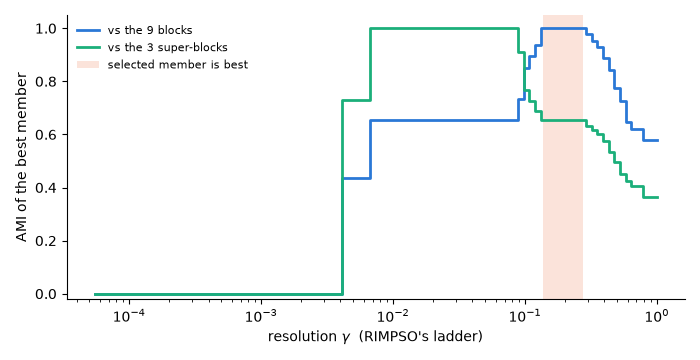The RIMPSO page gives the score. The figure below scores the best member at every rung against both planted partitions with pymocd.ami. The planted partitions serve here only for plotting and evaluation; the selection that rimpso_fronts returns does not use them.

ami_blocks = np.array([pymocd.ami(p, blocks) for p in partitions])
ami_super = np.array([pymocd.ami(p, super_blocks) for p in partitions])

fig, ax = plt.subplots(figsize=(7, 3.6))
ax.plot(gammas, ami_blocks[best], color=BLUE, lw=2, drawstyle="steps-mid", label=f"vs the {n_blocks} blocks")
ax.plot(gammas, ami_super[best], color=AQUA, lw=2, drawstyle="steps-mid", label=f"vs the {n_super} super-blocks")
if on_selected.any():
    ax.axvspan(gammas[on_selected].min(), gammas[on_selected].max(), color=ORANGE, alpha=0.18, lw=0,
               label="selected member is best")
ax.set_xscale("log")
ax.set_ylim(-0.02, 1.05)
ax.set_xlabel(r"resolution $\gamma$  (RIMPSO's ladder)")
ax.set_ylabel("AMI of the best member")
ax.legend(loc="upper left", fontsize=8, frameon=False)
ax.spines[["top", "right"]].set_visible(False)
fig.tight_layout()
plt.show()

if on_selected.any():
    lo, hi = gammas[on_selected].min(), gammas[on_selected].max()
    print(f"selected member is best on {on_selected.sum()} rungs, gamma in [{lo:.4g}, {hi:.4g}]")
else:
    print("selected member is best on no rung of the ladder")
print(f"AMI of the selected member: {ami_blocks[selected]:.3f} vs the blocks, "
      f"{ami_super[selected]:.3f} vs the super-blocks")
print(f"highest AMI on the front:   {ami_blocks.max():.3f} vs the blocks, "
      f"{ami_super.max():.3f} vs the super-blocks")

plot resolution profile

Out:

selected member is best on 8 rungs, gamma in [0.1378, 0.2758]
AMI of the selected member: 1.000 vs the blocks, 0.653 vs the super-blocks
highest AMI on the front:   1.000 vs the blocks, 1.000 vs the super-blocks

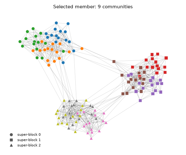
Draw the selected partition¶

Node color is the selected community; node shape is the planted super-block.

chosen = partitions[selected]
order = {}
for v in sorted(chosen):
    order.setdefault(chosen[v], len(order))  # color communities in order of their lowest node

pos = nx.spring_layout(G, seed=3)
cmap = plt.colormaps["tab10"]
fig, ax = plt.subplots(figsize=(6, 5))
nx.draw_networkx_edges(G, pos, ax=ax, width=0.5, alpha=0.2)
for s, marker in zip(range(n_super), ["o", "s", "^"]):
    nodes = [v for v in G if super_blocks[v] == s]
    nx.draw_networkx_nodes(
        G, pos, nodelist=nodes, node_shape=marker, node_size=55,
        node_color=[cmap(order[chosen[v]]) for v in nodes],
        edgecolors="white", linewidths=0.5, ax=ax,
    )
handles = [
    plt.Line2D([], [], marker=mk, linestyle="", color="0.35", label=f"super-block {s}")
    for s, mk in zip(range(n_super), ["o", "s", "^"])
]
ax.legend(handles=handles, loc="lower left", fontsize=8, frameon=False)
ax.set_title(f"Selected member: {k[selected]} communities", fontsize=11)
ax.set_axis_off()
fig.tight_layout()
plt.show()

Selected member: 9 communities

To apply the same selector to a front that another detector produced, see Choosing a partition from a front.

Total running time of the script: ( 0 minutes 0.542 seconds)

Download Python source code: plot_resolution_profile.py

Download Jupyter notebook: plot_resolution_profile.ipynb

Gallery generated by mkdocs-gallery