Recovery as mixing increases¶

Generate planted-partition graphs from well-separated to nearly random, run pymocd.rimpso, pymocd.hpmocd and pymocd.gdpso on each one, and plot how closely each detector recovers the planted blocks as the mixing grows.

Graphs with a controlled mixing level¶

Every graph comes from nx.planted_partition_graph with l = 6 blocks of k = 50 nodes (n = 300). For a target mixing mu and a target expected degree d = 16, the edge probabilities are

p_in = d * (1 - mu) / (k - 1) inside a block,
p_out = d * mu / (n - k) between blocks,

so a node expects d * (1 - mu) neighbors inside its block and d * mu outside it: the expected degree stays at d, the expected fraction of edges between blocks is mu, and only the mixing changes. Each target is drawn with three graph seeds. The mixing used on the plot is the realized one, counted on the edges of each generated graph.

import matplotlib.pyplot as plt
import networkx as nx
import numpy as np

import pymocd

BLOCKS, SIZE, DEGREE = 6, 50, 16
N = BLOCKS * SIZE
TARGETS = [0.1, 0.2, 0.3, 0.4, 0.5, 0.6, 0.7, 0.8]
SEEDS = [1, 2, 3]


def planted(mu, seed):
    """A planted-partition graph, its blocks, and its realized mixing."""
    p_in = DEGREE * (1 - mu) / (SIZE - 1)
    p_out = DEGREE * mu / (N - SIZE)
    G = nx.planted_partition_graph(BLOCKS, SIZE, p_in, p_out, seed=seed)
    truth = {v: b for b, block in enumerate(G.graph["partition"]) for v in block}
    mixing = sum(truth[u] != truth[v] for u, v in G.edges()) / G.number_of_edges()
    return G, truth, mixing


def louvain(graph):
    """NetworkX Louvain, returned in pymocd's {node: community} form."""
    communities = nx.community.louvain_communities(graph, seed=1)
    return {v: c for c, members in enumerate(communities) for v in members}

Run the sweep¶

Each detector runs at its default parameters, once per graph, and pymocd.ami scores its partition against the planted blocks. NetworkX's Louvain implementation with a fixed seed is included as an external reference point.

detectors = {
    "rimpso": pymocd.rimpso,
    "hpmocd": pymocd.hpmocd,
    "gdpso": pymocd.gdpso,
    "Louvain (networkx)": louvain,
}

mixing = np.zeros((len(TARGETS), len(SEEDS)))
ami = {name: np.zeros((len(TARGETS), len(SEEDS))) for name in detectors}
for i, mu in enumerate(TARGETS):
    for j, seed in enumerate(SEEDS):
        G, truth, mixing[i, j] = planted(mu, seed)
        for name, detect in detectors.items():
            ami[name][i, j] = pymocd.ami(detect(G), truth)

Plot recovery against the realized mixing¶

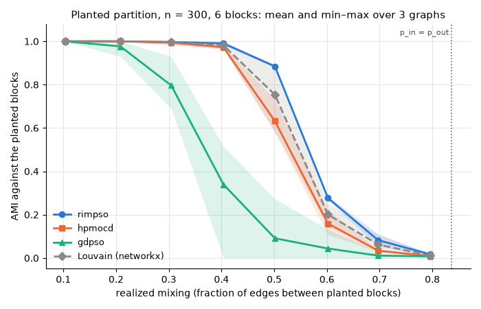
Each line joins the mean AMI over the three graphs at one target mixing, placed at their mean realized mixing; the shaded band spans the lowest and highest AMI of the three. The dotted vertical line marks the expected mixing at which p_in = p_out, that is mu = (n - k) / (n - 1): there two nodes are as likely to be linked across blocks as inside one, and the graph carries no trace of the planted blocks.

style = {
    "rimpso": {"color": "#2a78d6", "marker": "o"},
    "hpmocd": {"color": "#eb6834", "marker": "s"},
    "gdpso": {"color": "#1baf7a", "marker": "^"},
    "Louvain (networkx)": {"color": "#8a8985", "marker": "D", "linestyle": "--"},
}

x = mixing.mean(axis=1)
fig, ax = plt.subplots(figsize=(7, 4.5))
for name, scores in ami.items():
    s = style[name]
    ax.fill_between(x, scores.min(axis=1), scores.max(axis=1), color=s["color"], alpha=0.15, linewidth=0)
    ax.plot(x, scores.mean(axis=1), label=name, linewidth=2, markersize=6, **s)
ax.axvline((N - SIZE) / (N - 1), color="0.4", linestyle=":", linewidth=1.2)
ax.text((N - SIZE) / (N - 1), 1.02, "p_in = p_out ", color="0.3", fontsize=8, va="bottom", ha="right")
ax.set_xlabel("realized mixing (fraction of edges between planted blocks)")
ax.set_ylabel("AMI against the planted blocks")
ax.set_ylim(-0.05, 1.08)
ax.grid(color="0.9")
ax.set_axisbelow(True)
ax.spines[["top", "right"]].set_visible(False)
ax.legend(frameon=False, fontsize=9, loc="lower left")
ax.set_title(f"Planted partition, n = {N}, {BLOCKS} blocks: mean and min–max over {len(SEEDS)} graphs", fontsize=11)
fig.tight_layout()
plt.show()

Planted partition, n = 300, 6 blocks: mean and min–max over 3 graphs

The numbers behind the plot¶

Mean AMI over the three graphs at each target mixing, next to the mean and range of the realized mixing.

columns = {"rimpso": "rimpso", "hpmocd": "hpmocd", "gdpso": "gdpso", "Louvain (networkx)": "Louvain"}
print(f"{'target':>6}  {'realized mixing':<21}" + "".join(f"{label:>9}" for label in columns.values()))
for i, mu in enumerate(TARGETS):
    realized = f"{x[i]:.3f} [{mixing[i].min():.3f}, {mixing[i].max():.3f}]"
    print(f"{mu:>6.1f}  {realized:<21}" + "".join(f"{ami[name][i].mean():>9.3f}" for name in columns))

Out:

target  realized mixing         rimpso   hpmocd    gdpso  Louvain
   0.1  0.103 [0.097, 0.108]     1.000    1.000    1.000    1.000
   0.2  0.208 [0.203, 0.216]     1.000    1.000    0.977    1.000
   0.3  0.305 [0.294, 0.313]     0.997    0.994    0.796    0.997
   0.4  0.404 [0.400, 0.407]     0.991    0.973    0.340    0.981
   0.5  0.501 [0.499, 0.504]     0.885    0.632    0.091    0.754
   0.6  0.602 [0.594, 0.611]     0.277    0.159    0.044    0.201
   0.7  0.697 [0.695, 0.699]     0.082    0.034    0.011    0.062
   0.8  0.796 [0.783, 0.803]     0.017    0.009    0.008    0.011

Reading the sweep¶

An AMI near 1 means the planted blocks were recovered; an AMI near 0 means the partition agrees with them no more than chance would, and a partition that puts every node in one community scores exactly 0. Look at the mixing at which each curve starts to fall and at the width of its band: a wide band means the outcome depends on the particular graph and, for a nondeterministic detector, on the run. The module READMEs describe rimpso and gdpso as deterministic and hpmocd as nondeterministic, so the hpmocd curve can change from one build of this page to the next.

The detectors optimize different things: rimpso searches the Constant Potts Model's resolution profile, hpmocd a bi-objective split of modularity, and gdpso modularity alone (see the algorithms overview). The sweep is small, one graph size with three seeds per level, so it is sized to run while the documentation builds, not to rank detectors. Comparing detectors runs all ten detectors on a single graph, and Evaluating partitions explains AMI and the other metrics.

Total running time of the script: ( 0 minutes 14.832 seconds)

Download Python source code: plot_mixing_sweep.py

Download Jupyter notebook: plot_mixing_sweep.ipynb

Gallery generated by mkdocs-gallery