Comparing detectors on a planted partition¶

Generate a graph whose communities are planted by construction, run all ten detector entry points at their default parameters, and compare the partition each one returns with the planted blocks and the wall time it takes.

A graph with known communities¶

nx.planted_partition_graph(l, k, p_in, p_out, seed=...) splits l * k nodes into l blocks of k nodes and joins each pair of nodes with probability p_in if they share a block and p_out otherwise. NetworkX stores the blocks in the graph attribute G.graph["partition"], which serves as ground truth here.

The mixing of the graph is the fraction of its edges that join two different blocks. It is counted on the edges the generator actually drew, so it is the realized value for this graph, not the expected value implied by p_in and p_out.

import time

import matplotlib.pyplot as plt
import networkx as nx

import pymocd

G = nx.planted_partition_graph(6, 50, 0.2, 0.025, seed=7)
truth = {v: b for b, block in enumerate(G.graph["partition"]) for v in block}

m = G.number_of_edges()
between = sum(truth[u] != truth[v] for u, v in G.edges())
print(f"{G.number_of_nodes()} nodes, {m} edges, {len(G.graph['partition'])} planted blocks")
print(f"realized mixing: {between / m:.3f} ({between} of {m} edges join two blocks)")

Out:

300 nodes, 2325 edges, 6 planted blocks
realized mixing: 0.397 (922 of 2325 edges join two blocks)

Run every detector¶

Each detector runs once with its own default parameters and is timed with time.perf_counter. pymocd.ami scores the partition it returns against the planted blocks (1 is a perfect match, 0 is the agreement expected by chance). The library's own methods are pymocd.rimpso and pymocd.hpmocd; the other eight entry points are re-implemented baselines (Shi-MOCD has two, mocd_q and mocd_d), described in the algorithms overview. NetworkX's Louvain implementation, nx.community.louvain_communities with a fixed seed, is added as an external reference point.

The first parallel call in a process builds the Rayon thread pool (Performance and reproducibility), so one untimed call on a small graph comes first; otherwise that one-time cost would be charged to whichever detector is timed first.

def louvain(graph):
    """NetworkX Louvain, returned in pymocd's {node: community} form."""
    communities = nx.community.louvain_communities(graph, seed=1)
    return {v: c for c, members in enumerate(communities) for v in members}


detectors = {
    "rimpso": pymocd.rimpso,
    "hpmocd": pymocd.hpmocd,
    "cdrme": pymocd.cdrme,
    "mmcomo": pymocd.mmcomo,
    "ccm": pymocd.ccm,
    "krm": pymocd.krm,
    "gdpso": pymocd.gdpso,
    "mocd_q": pymocd.mocd_q,
    "mocd_d": pymocd.mocd_d,
    "moga_net": pymocd.moga_net,
    "Louvain (networkx)": louvain,
}

pymocd.rimpso(nx.karate_club_graph())  # untimed warm-up

results = {}
for name, detect in detectors.items():
    start = time.perf_counter()
    partition = detect(G)
    seconds = time.perf_counter() - start
    results[name] = {
        "k": len(set(partition.values())),
        "ami": pymocd.ami(partition, truth),
        "seconds": seconds,
    }

Plot AMI and wall time¶

Both panels list the detectors in the same fixed order: the two pymocd methods, the eight baseline entry points, then the external reference.

own = {"rimpso", "hpmocd"}
reference = {"Louvain (networkx)"}
group_color = {"pymocd method": "#2a78d6", "re-implemented baseline": "#eb6834", "external reference": "#8a8985"}


def group(name):
    if name in own:
        return "pymocd method"
    if name in reference:
        return "external reference"
    return "re-implemented baseline"


names = list(results)
rows = range(len(names))
colors = [group_color[group(name)] for name in names]
amis = [results[name]["ami"] for name in names]
times = [results[name]["seconds"] for name in names]

fig, (ax_ami, ax_time) = plt.subplots(1, 2, figsize=(10, 5), sharey=True)

bars = ax_ami.barh(rows, amis, color=colors, height=0.7)
ax_ami.bar_label(bars, fmt="%.2f", padding=3, fontsize=8, color="0.3")
ax_ami.set_xlim(min(0.0, min(amis)), 1.15)
ax_ami.set_xlabel("AMI against the planted blocks")

bars = ax_time.barh(rows, times, color=colors, height=0.7)
ax_time.bar_label(bars, fmt="%.2f s", padding=3, fontsize=8, color="0.3")
ax_time.set_xlim(0, max(times) * 1.25)
ax_time.set_xlabel("wall time (s), one run")

ax_ami.set_yticks(list(rows), names)
ax_ami.invert_yaxis()
for ax in (ax_ami, ax_time):
    ax.grid(axis="x", color="0.9")
    ax.set_axisbelow(True)
    ax.spines[["top", "right"]].set_visible(False)

handles = [plt.Rectangle((0, 0), 1, 1, color=c, label=g) for g, c in group_color.items()]
fig.legend(handles=handles, loc="lower center", ncol=3, frameon=False, fontsize=9)
fig.suptitle(f"Planted partition, {G.number_of_nodes()} nodes: default parameters, one run each", fontsize=12)
fig.tight_layout(rect=(0, 0.06, 1, 1))
plt.show()

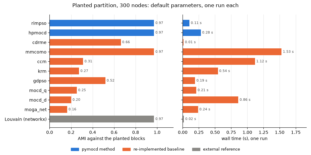
Planted partition, 300 nodes: default parameters, one run each

The numbers behind the plot¶

k is the number of communities in the returned partition; the planted graph has six.

print(f"{'detector':<20} {'k':>4} {'AMI':>7} {'seconds':>9}")
for name, r in results.items():
    print(f"{name:<20} {r['k']:>4} {r['ami']:>7.3f} {r['seconds']:>9.3f}")

Out:

detector                k     AMI   seconds
rimpso                  6   0.972     0.105
hpmocd                  6   0.972     0.281
cdrme                  15   0.663     0.014
mmcomo                  6   0.972     1.530
ccm                    16   0.312     1.118
krm                    20   0.274     0.544
gdpso                   2   0.519     0.192
mocd_q                  8   0.254     0.210
mocd_d                  4   0.201     0.861
moga_net               14   0.164     0.238
Louvain (networkx)      6   0.972     0.019

Reading the comparison¶

Timings are from the machine that built these docs. They depend on its processor and on the number of cores available, and each detector is timed once. Each time includes converting the NetworkX graph to the library's internal representation and building the returned dict, not only the search. Run the script on your own hardware before drawing conclusions about speed; Performance and reproducibility covers thread counts.
Each detector runs at its own defaults, so the time reflects each default budget (population size, number of generations), which differs from one detector to the next. The docstrings of pymocd.mocd_q and pymocd.mocd_d note that their defaults are the repository's benchmark budget, not the configuration published by Shi et al. (2012); see Shi-MOCD.
One partition per detector. Detectors that build a Pareto front return one member of it, chosen by a selection rule; the front itself can hold partitions that score differently. Where a *_fronts function exists, it returns the whole candidate set; see Working with Pareto fronts.
Some detectors are nondeterministic. The module READMEs describe rimpso, cdrme and gdpso as deterministic and the other seven entry points as nondeterministic, so their k and AMI values can change from one build of this page to the next.
One graph is one data point. This graph has a single size and a single mixing level. Recovery as mixing increases repeats the measurement across mixing levels and graph seeds, and Choosing a detector discusses which detector fits which task.

Total running time of the script: ( 0 minutes 5.327 seconds)

Download Python source code: plot_compare_detectors.py

Download Jupyter notebook: plot_compare_detectors.ipynb

Gallery generated by mkdocs-gallery